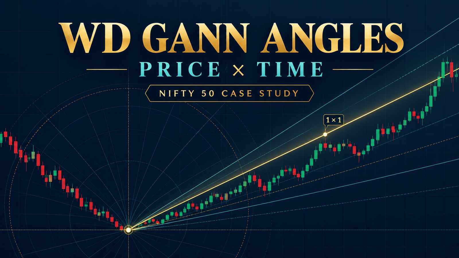
WD Gann’s Geometrical Angles: Meaning, Chart Setup and a Nifty Example

WD Gann’s geometrical-angle method is a way to study the relationship between price movement and time on a chart. Gann treated selected angles—especially the 1×1 angle—as reference lines for judging whether price was rising or falling at a particular pace. Traders who study the method may use the lines to observe trend strength and possible support or resistance areas.

These are chart-analysis ideas, not mathematical laws that guarantee market turns. The result depends on the chart’s time and price scales, the chosen starting point and the market data being studied.

1. The basic idea: represent price against time

A price chart already has two dimensions:

• The horizontal axis shows time: trading sessions, weeks or months.
• The vertical axis shows price: rupees, index points or another unit.

A trend line drawn from a major high or low shows how price changed over time from that point. Gann’s method gives particular slopes names such as 1×1, 2×1 and 1×2.

In the traditional interpretation, a 1×1 line advances one price unit for each time unit. For example, if one time unit is one trading session and one price unit is 100 index points, the line rises 100 points per session. A 45-degree appearance is produced only when the chart’s horizontal and vertical scales are set so that the selected price and time units occupy equal chart distances.

That scaling condition matters: a line that looks like 45 degrees on one chart may not look like 45 degrees after the chart is resized or the price axis is changed.

2. What the circle’s 360 degrees mean

A full circle contains 360 degrees. In Gann-style studies, chart users may divide the circle into portions—such as 45°, 90° or 180°—and investigate whether those divisions have coincided with price or time events in historical data.

The geometric fact is that a circle has 360 degrees. The further claim—that specific angles consistently identify market tops, bottoms or resistance—is a market-analysis hypothesis. It must be tested against data; the number 360 alone does not establish that a reversal will occur.

3. Common angle ratios

A ratio describes how much price changes for a chosen amount of time:

Traditional angle	Example if 1 time unit = 1 session and 1 price unit = 100 points
1×1	100 points per session
2×1	200 points per session
1×2	50 points per session

In the traditional reading, a rising price line that stays above a rising 1×1 reference is considered to be moving upward faster than that reference. A move below it may indicate that the rise has slowed relative to the line. These are interpretations of the selected chart model, not guarantees of a future move.

The scale is part of the method. Before comparing angles, specify the time unit, price unit, chart type and starting pivot. Otherwise two people can draw different “1×1” lines on the same price history.

4. Why geometry does not replace calculation

The passage you described argues that accurately drawn angles can expose addition or multiplication mistakes. A chart can help a researcher spot an inconsistency, but drawing a line does not automatically correct a calculation error.

For a reproducible study, record the numerical inputs as well as the visual line:

1. Choose a clear high or low as the starting pivot.
2. Choose a time unit, such as one trading session.
3. Choose a price unit, such as 100 Nifty points.
4. Calculate each line’s price level at each elapsed time unit.
5. Compare those levels with actual price data.

This makes the method easier to audit and back-test than relying on how steep a line looks on screen.

5. Worked Nifty example: 7 April 2025 low

The Nifty 50 recorded an intraday low of 21,743.65 on 7 April 2025 and closed that session at 22,161.60. On 8 April, it closed at 22,535.85.

For a simple angle exercise, set:

• Starting pivot: 21,743.65 on 7 April 2025
• Time unit: one trading session
• Price unit: 100 Nifty points
• Reference line: rising 1×1

Using that chosen scale, the reference line would be:

Sessions after pivot	1×1 reference level
0	21,743.65
1	21,843.65
2	21,943.65
3	22,043.65
4	22,143.65

The 8 April close was 22,535.85—about 792 points above the 7 April low, while the example 1×1 line after one session is 21,843.65. This shows that the market’s rebound was much faster than this particular reference line over that interval. It does not prove that the 1×1 scale was the correct one or that the line predicted the rebound. Another choice of price unit would produce a different comparison.

That is why a good study states its scale in advance and tests it on many past periods, including periods where the line did not appear to work.

6. Moving averages: an important distinction

A standard simple moving average (SMA) is the average of a selected number of closing prices:

SMA = sum of the closing prices over the selected periods ÷ number of periods

For example, the Nifty’s closes from 1–7 April 2025 were 23,165.70, 23,332.35, 23,250.10, 22,904.45 and 22,161.60. Their five-session simple moving average is 22,962.84.

A midpoint calculated from the high and low is a different measure. On 7 April, the day’s high was 22,254 and low was 21,743.65, giving a high-low midpoint of about 21,998.83. That is not the same as a five-session moving average.

So if a passage describes averaging a period’s high and low, it is useful to identify exactly which calculation it means. Don’t treat a high-low midpoint, moving average and Gann angle as interchangeable indicators.

7. A practical way to study the method

To evaluate geometrical angles as a research tool:

• Use the same chart type and price scale throughout the test.
• Select pivots using a rule written before looking at the outcome.
• Record the angle’s projected price level for each time step.
• Compare the line with actual prices, including false signals and failed holds.
• Test separate samples, rather than selecting only examples that fit the theory.
• Include other market information and risk limits in any trading decision.

Conclusion

Gann’s geometrical angles provide a structured way to compare price movement with elapsed time. Their usefulness depends on clearly defined units, consistent chart scaling and evidence from historical testing. The 360-degree circle and a drawn 45-degree line are geometric constructions; they do not, by themselves, establish that a market will reverse or continue in a particular direction.

This article is for education and research only. It is not investment advice or a recommendation to buy or sell. Past market examples do not predict future results.